What is physical intuition?

How can qualitative physical understanding help us solve problems? When does it work and fail?

Leveraging physical understanding

One thing that I’ve been interested in for some time is trying to understand solutions to complicated equations at an intuitive level. This is particularly relevant in physics because the equations that we encounter pertain to things in the natural world, and a good “understanding” of the equation necessitates a good grasp of the physical concepts. This is what Paul Dirac, one of the greatest physicists of the 20th century, had to say about understanding equations:

“I consider that I understand an equation when I can predict the properties of its solutions, without actually solving it.”
Paul Dirac

What could this mean? How is it possible to understand the properties of an equation’s solutions without actually solving it? As a basic example of this, suppose I asked you to solve the following integral:

\[I:= \int\limits_{0}^{\infty} \left( \frac{m}{2 \pi k_B T} \right)^{\frac{3}{2}} 4\pi v^2 e^{-\frac{mv^2}{2 k_B T}} \text{d}v\]

If you don’t recognise this integrand, a reasonable approach would be to just go ahead with some algebra. In fact, if you know a bit about Gaussian integrals, this isn’t a particularly challenging problem. But before you demonstrate your finely-tuned integration skills, let’s pause for a moment - with a bit of extra information about the system, we can use our physical intuition to determine the answer to this integral without any calculation.

The first question to ask is, “what is this equation describing?”. If we inspect the terms, we find that $m$ is mass of particles, $k_B$ is the Boltzmann constant, $T$ is temperature of a gas, and $v$ is the speed of each particle. In addition, the integral goes from $0$ to $\infty$, integrating over the particle speeds.

If you haven’t already guessed, this describes a probability distribution over the speeds of particles in an ideal gas¹. Once we know this, the answer becomes clear! Imagine a box filled with particles bouncing around like billiard balls. These particles have different speeds, which we can describe using a distribution.

The integral tells us the probability that each particle in the gas has any speed from 0 to $\infty$, which is clearly 1. You can verify this by doing integration by parts².

With a touch of physical understanding we were able to get to the solution without actually solving it! The benefits of understanding what the equation describes don’t just stop there - it also allows us to check whether or not the integrand itself makes sense in the first place. Essentially, the question is this: we’ve solved the integral and gotten a reasonable answer, but why should the probability distribution take this form? To answer this, let’s break down the integrand $p(v)$:

\[p(v) = \left( \frac{m}{2 \pi k_B T} \right)^{\frac{3}{2}} 4\pi v^2 e^{-\frac{mv^2}{2 k_B T}}.\]

The probability that a gas particle has a speed that lies within a particular range is found (as we saw) by integrating over the speeds. This depends on two key variables:

• Particle mass $m$: intuitively we would expect that heavier particles should move slower than lighter particles.
• Temperature $T$: roughly this is an average measure of the speeds of the gas particles. If we increase the temperature, we’d expect that on average the each particle is more likely to move faster.

If you try and compare your physical intuition with what the equation is showing, it can be quite difficult to tell exactly what the behaviour will be like. Even if you recognise that the exponential term dominates the function’s behaviour at large speeds, when exactly it becomes the dominant contributor can be hard to discern. To try and get a better feel for this, let’s take a look at the graph of this.

If you increase the temperature then the peak of the distribution shifts to the right, meaning that the particles on average have a higher speed. You can try having a fiddle around with the controls in the GeoGebra applet and see if you can justify to yourself why this behaviour makes sense - for example, what happens if you increase the mass? Does this agree with what you expect?

From this simple example we can see that having a grasp of the physics gives an understanding of the situation that would allow us to make predictions about how the system should behave. Therefore, what I mean by having “physical understanding” or “physical intuition” is this: having the ability to understand a system based on a mental physical model, as opposed to grinding through equations.

Simplifying assumptions

This one has become a bit of a joke, even among physicists! The classic example of is this: to determine how much heat gets radiated from a cow, the first simplifying step is to “imagine a spherical cow”³, which is only “a bit” of a caricature of what cows actually look like.

Let’s continue the example from the previous section. Suppose we’re trying to model the behaviour of a real gas (say the box is filled with air), what assumptions have we made? (Go back and have a look, the assumptions were introduced in rather sneaky fashion.)

If you’re a really careful reader, you’ll notice that the Maxwell-Boltzmann distribution describes the behaviour of an ideal gas. This is loaded with simplifications! For instance:

• Gas particles can be thought of as point particles, such that they don’t take up any space
• There are no interactions between particles apart from collisions
• The particle collisions are perfectly elastic, such that the total kinetic energy of the gas in the box stays the same

Another simplification is that there are a sufficiently large number of particles, such that we can define properties like “temperature”, and model the system using a statistical distribution.

On the outset, these assumptions might seem quite sketchy, so why might it be reasonable to do so?

• Point particles: This assumption is actually made relative to the environment - gas particles are typically very small, on the order of $\approx 10^{-10}$ metres in diameter. In contrast, if we think of a “box” of particles, we’re typically thinking of things that are at macroscopic scales, on the order of a metre in length. This is a huge difference, and to us they seem basically like points.
• No interparticle forces: Related to the previous assumption, is that the particles don’t form any intermolecular bonds. This seems pretty consistent with what one might expect from the kinetic theory of matter, where solids have strong interparticle bonds and gas particles have very weak ones (such that they can move around independently).
• Elastic collisions: If particles ever collide with the containing box, we’re assuming that the box never changes in energy and that the particles maintain their speed. If particles collide with each other, the total kinetic energy is the same before and after collisions. This lets us focus on the “average” behaviour of the system over time⁴.
• Many particles: Gases in general have lots of particles in them - for instance, at standard temperature and pressure there are close to $10^{22}$ particles per litre of oxygen⁵. This is nice if we want to take a statistical approach to analysing the system, as we’ve seen in the previous section.

In essence, these assumptions make things much easier to handle without losing too much explanatory power.

I think the extent of the simplifications probably depends on how well you understand the physical system that you’re interested in. If you have no idea where to start, I think it really does make sense to just simplify things and then “see how things go”. This can often yield very good results, because not every physical characteristic of the system you’re interested in is super relevant. If the simplification only leaves behind useful stuff, then you probably already have a pretty good approximation for how things work in reality. This is why classical Newtonian gravity can be highly useful, even though technically General Relativity gives a better description of reality. Relativity gives us more explanatory power overall, but it’s a lot more fiddly and simply not necessary in everyday situations.

A corollary of this is that breaking your previous simplifying assumptions is plausibly a great way to make progress - in fact, I think a lot of modern physics research is in this vein. For instance, the fourth assumption from earlier assumes that the box has many gas particles (e.g. $n \approx 10^{22}$). If we imagine the spectrum of systems of particles that physicists tend to think about, this would be at one extreme, and at the other extreme we have systems with very few (e.g. $n = 1,2$) particles. Both of these cases are well understood, with statistics helping in the former and the basic laws of physics easily applying in the latter. What’s challenging is the cases in between, with say $n = 20$ to $50$ particles - now we’re suddenly at the forefront of condensed matter, where researchers deal with quantum dots, which contain a comparable number of electrons. In this sense, simplifications can make our lives a lot easier, and also suggest further paths for investigation.

Dimensional Analysis

Of course, even when we’re armed with information about the system, knowing the properties of the solutions isn’t always an easy thing to do! Fortunately, we have more tricks up our sleeve. In the previous example we started off by looking at what the symbols describe - we can add a level of nuance to this by looking at their dimensions (e.g. momentum $p$ has dimensions of $\text{mass} * \text{length} * \text{time}^{-1} $). A stronger form of this involves looking at the units (e.g. one possible unit of momentum is $\text{kilograms} * \text{metres} / \text{second}$).

This can be used if we want to check that our equations make sense, by comparing the dimensions on the left and right hand sides of each equation⁶. Looking at units is also very important, not just in exams but also in ensuring that you don’t accidentally crash Mars Climate Orbiters (dear reader, please use metric units in science).

In some cases we can do even better - rather than just using dimensional analysis as a sanity check, we can use it to predict what our solutions might look like. A great example of this is given by John Adam in Mathematics in Nature, which makes a dimensional argument as to why the sky should be blue.

Why the sky is blue seems like a surprisingly difficult question to answer, so let’s try and break it down a bit. What we do know is that light from the sun comes in a spectrum, which to the naked eye looks roughly white. Through some process of interaction with the particles in the atmosphere, the light that reaches our eyes is blue.

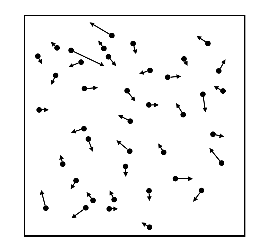
What is this interaction? If we take a random patch of atmosphere and zoom in really close, we’ll find that it consists of lots of small gas molecules, mainly Nitrogen and Oxygen. As we discussed earlier, these have length on the order of $10^{-10}$ metres. At the same time, visible light from the sun has a wavelength of about $10^{-7}$ metres, a factor of about a thousand. Unlike in the previous section, things start to become a little ambiguous - should we still treat these gas molecules as point particles?

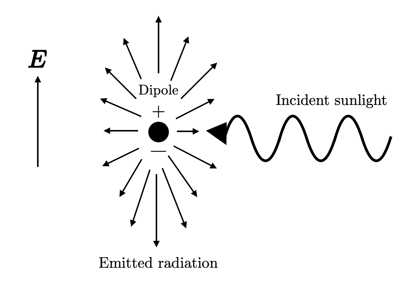
The important consideration here is that these particles often are likely to interact with light through charge separation (since light is an electromagnetic field), where positive charges get pushed in the direction of the electric field, and negative charges in the opposite direction. This forms an oscillating dipole, releasing radiation. As a result, one might expect that the wavelength is quite important here - the shorter the wavelength of incident sunlight, the higher the oscillation frequency.

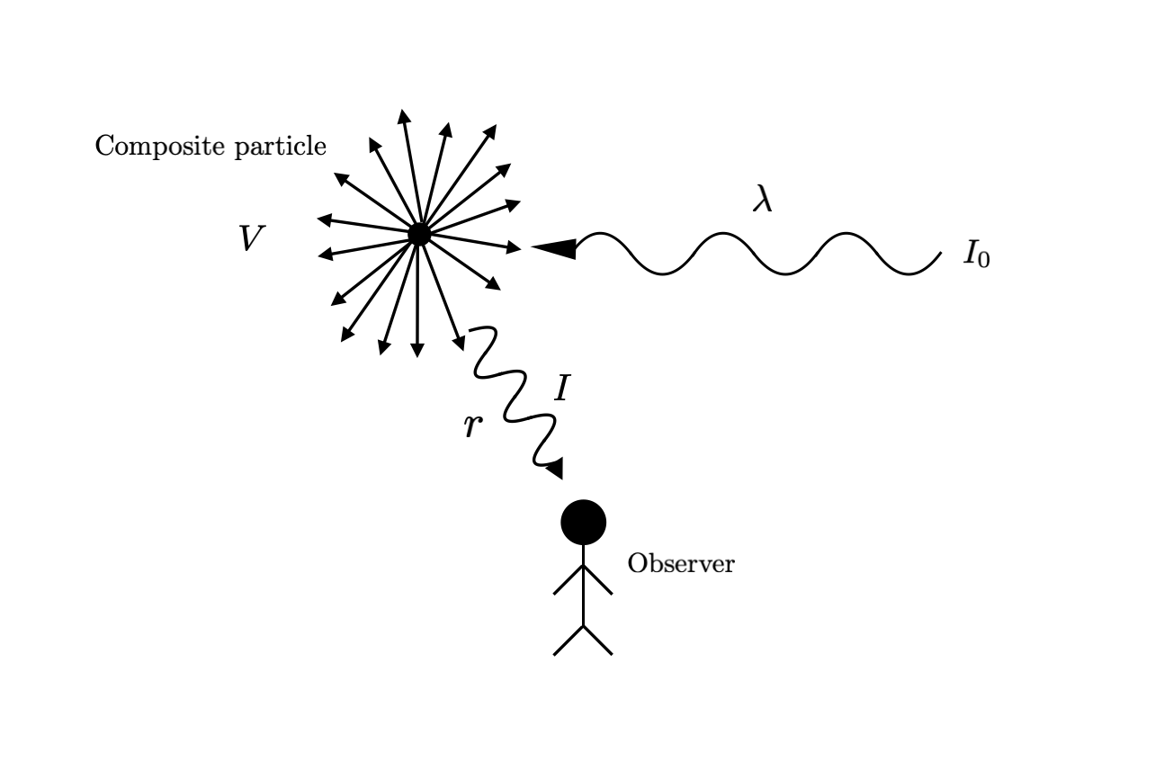
One might also guess that this increased frequency results in emitted radiation of a higher frequency. To check this, let’s think about the intensity of the emitted radiation that an observer sees. Intuitively, this probably depends on several factors:

• The number of particles $N$ - we can think of these as forming a “composite particle” in 3D space consisting of the particles that scatter light into the observer’s eyes. Let’s call the volume of this composite particle $V$
• The distance from the composite particle to the observer $r$
• The wavelength of incident light $\lambda$
• The intensity of incident light $I_0$

Let’s rewrite the above in mathematical form - if the emitted radiation has intensity $I$, then it is a function of the above factors:

\[I = f(V, r, \lambda, I_0).\]

Now comes the dimensional analysis. From the equation above, we substitute in constants for the powers:

\[I \propto V^\alpha r^\beta \lambda^\gamma I_0.\]

If we do dimensional analysis on this, then we notice that $V$, $r$ and $\lambda$ have dimensions of $[\text{Length}]^3$, $[\text{Length}]$ and $[\text{Length}]$ respectively. The two intensities have the same dimensions, and thus we have

\[[\text{Length}]^{3\alpha}[\text{Length}]^\beta[\text{Length}]^\gamma = [\text{Length}]^0.\]

What we need now is two extra pieces of physical information that tell us what values these constants $\alpha, \beta, \gamma$ take.

• First, we know that the amplitude of radiation is proportional to the number of scatterers (electric fields supoerpose linearly), which is in turn proportional to $V$. Since intensity is proportional the square of the amplitude, we have $\alpha = 2$
• Second, we should expect the radiation intensity to decrease inversely as the square of the distance (i.e. as $\frac{1}{r^2}$) Why? Far away from the dipole, the emitted radiation looks like it’s spread out over a sphere - the intensity of this light decreases at the rate at which the area increases, and since the area of the sphere is $4\pi r^2$ the result follows. Thus $\beta = -2$.

Substituting this back into the proportionality relation suggests that $\gamma = -4$, and thus $I \propto \lambda^{-4}$.

Now we have everything we need to answer the original question. We’ve just shown that light of a longer wavelength tends to have scattered light of a lower intensity, and this dependence is strong - slightly longer wavelengths are probably going to lead to significantly weaker emitted radiation. At the same time, we also know blue light has a shorter wavelength, so this relation tells us that blue light is scattered much more strongly in the atmosphere than other colours, and thus the sky appears blue⁷.

I think this is argument is quite remarkable! The usual approach requires slogging through Maxwell’s equations, but the dimensional argument circumvents these tedious steps - who would’ve thought?

Checking equations

Another way of getting a better grip over opaque-seeming equations is to look at its behaviour at certain extremes, and using our physical understanding to see if they make sense. Consider a charged circular disk in the $x-y$ plane centred at the origin with a radius $a$, which is uniformly charged with a charge density (charge per unit area) $\sigma$.

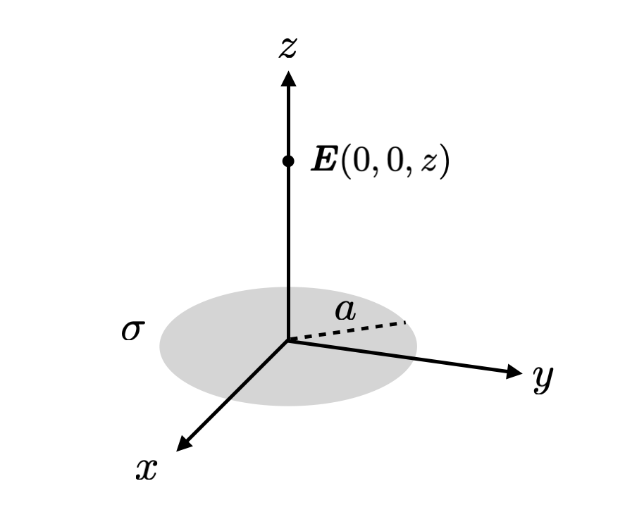
Now suppose I tell you that the electric field at some point $(0,0,z)$ on the $z$-axis has an electric field of

\[E(0,0,z) = \frac{\sigma}{2 \epsilon} \left\{1 - \frac{z}{\sqrt{a^2 + z^2}} \right\},\]

where $\epsilon$ is the permittivity (which for the purposes of this example you can think of as just a constant).

We now apply a series of sanity checks:

• First of all, the electric field should be symmetric with respect to the $z$ axis, because the charges in the system are too. Thus it must be pointing along the $z$ axis, and the equation should have no dependence on $x$ or $y$. Check!
• If the disc is positively charged, then the electric field should be point in the positive $z$ direction if $z>0$, and in the negative direction if $z < 0$. Whether this is satisfied is completely determined by the charge density $\sigma$, since the term in curly brackets is always positive if $a > 0$. When the plate is positively charged $\sigma > 0$, then $E(0,0,z) > 0$ as expected, and we can do a similar analysis in other cases. Check!
• As $z \to 0$, we have $E(0,0,0) \to \frac{\sigma}{\epsilon}$ - this matches our expectations for the electric field from a charged plane, and is what the field should “look like” locally, very close to the disc⁸. Check!
• As $z \to \infty$, the term in the curly brackets approaches 0, and thus the electric field tends to zero. This again matches our expectations, because the electric field from a charged plate infinitely far away should be close to zero. Check!

We can also try to be more nuanced with our analysis and describe what happens for large but finite $z$. The trick is to do a Taylor series expansion⁹, which you can show to be

\[E(0,0,z) = \frac{\sigma}{2 \epsilon} \left\{1 - \left\{ 1 - \frac{1}{2} \left( \frac{a}{2} \right)^2 + ...\right\} \right\}.\]

If we only pay attention to the lowest order terms (higher order terms will go to zero since $z$ is large¹⁰), then we see that

\[E(0,0,z) \approxeq \frac{\sigma_0 a^2}{4 \epsilon z^2} = \frac{\sigma_0 \pi a^2}{4 \pi \epsilon z^2} = \frac{Q}{4 \pi \epsilon z^2},\]

which is just what Coulomb’s law tells us is the electrostatic field from a point charge. This makes sense, because when we’re very far away from the disc such that $|z| » a$, the disc looks like a point. Check!

Thus the equation has passed all of the sanity checks, and it seems pretty likely that it correctly describes the electric field at $(z,0,0)$. We could also have applied other techniques that we’ve already seen, like dimensional analysis, to this problem. While these “tricks” don’t guarantee that your solution is correct, in my experience it does catch mistakes really often, and it is typically worth thinking about at least briefly.

Symmetries and abstraction

Another really powerful tool in a physicist’s toolbox is to look at the symmetries of a system, and tell you what form your equations should have as a result. Let’s take the example of the temperature of a metal rod:

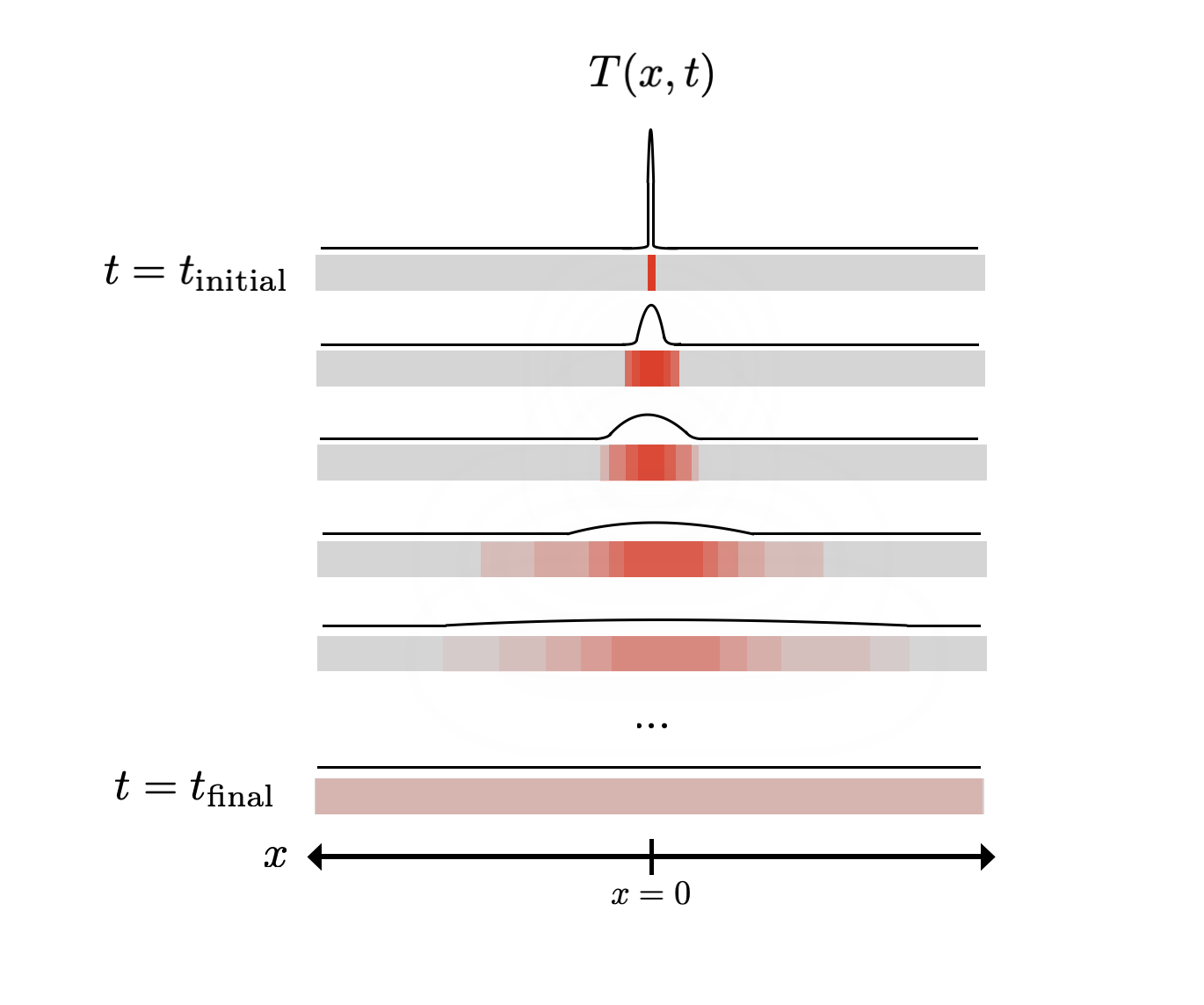
Suppose we heat the rod at the centre, which we’ll label as $x = 0$. What’s going to happen to the rod next? Even if you’ve never thought about this problem before, you probably have some intuition for this. The heat spreads over some period of time, and probably eventually evens out. Moreover, you never see this process running in reverse - the rod never goes from having a uniform temperature to being hot at a single point.

If we also think in terms of the spatial behaviour, then if we have a homogeneous material, there shouldn’t be any particular preference for the heat to spread in any direction (in the 1D case, heat shouldn’t preferentially spread either to the left $x < 0$ or to the right $x > 0$).

How do we translate what we’ve just said into an equation? The claims in the last two paragraphs are really statements about the rates of change of the system under one variable; i.e. partial derivatives. If we call the temperature of the rod $T$, which is a function of the time $t$ and the position $x$, then we’re interested in forming a partial differential equation with $T, \frac{\partial T}{\partial t}, \frac{\partial T}{\partial x}, \frac{\partial^2 T}{\partial t^2}, \frac{\partial^2 T}{\partial x^2}, \frac{\partial^2 T}{\partial t \partial x}, …$

Which of these terms can we rule out? We argued that $T(t)$ shouldn’t give the same result as $T(-t)$, so that means that we’re only interested in derivatives of $T$ that are of odd order - i.e. $\frac{\partial T}{\partial t}, \frac{\partial^3 T}{\partial t^3},$ and so on. Similarly, we argued that “left” or “right” has no physical significance, and so at any instant, $T(x) = T(-x)$ ¹¹. If we want this property to be true, then we rule out all of the derivatives of odd order, leaving us with $T, \frac{\partial^2 T}{\partial t^2}$, and so on.

Should we expect to see a term that depends directly on the temperature distribution $T$ in the PDE? Since we’re describing heat transfer, what’s important is differences in temperature, so the value of $T$ itself shouldn’t matter, and we can discard this term too.

Now we appeal to simplicity, and consider the most basic possible scenario that satisfies the previous conditions. That is, we want to relate just the lowest order derivatives possible, $\frac{\partial T}{\partial t}$ and $\frac{\partial^2 T}{\partial x^2}$ in a PDE. This gives us

\[\frac{\partial T}{\partial t} = D \frac{\partial^2 T}{\partial x^2},\]

where $D$ is a constant.

If you’re familiar with differential equations, you’ll recognise this as the heat equation or diffusion equation (here $D$ is known as the diffusion constant). This describes particles in a gas, electrons in semiconductors, and more!

Let’s reflect on what we just did. Through symmetry arguments, we were able to “derive” (albeit non-rigorously) an equation that has a ton of explanatory power¹². The symmetries that we considered were:

• Time-reversal symmetry: The system is fundamentally the same if $t \mapsto -t$ (which doesn’t apply to the metal rod)
• Parity: The system is fundamentally the same if we reflect space around the origin, i.e. if $x \mapsto -x$ (which applies to the metal rod)
• Isotropy: The system is fundamentally the same in all directions - this is subtly different from the previous one, in that we’re rotating space rather than reflecting it. The difference is perhaps better illustrated by going up to 2D - imagine a metal plate rather than a metal rod, in the $x-y$ plane. Then if the origin is heated, the heat spreads evenly in all directions. An isotropic system would “look the same” even if the axes were rotated, and a system with parity would “look the same” if one of the axes were flipped. In this case, the diffusion equation would have $\frac{\partial^2}{\partial x^2}$ be replaced by a Laplacian.

Many PDEs in physics can be described using similar symmetry arguments, like the Schrödinger and wave equations. I encourage you to try seeing how these arguments apply in those circumstances too.

If you’re a mathematician, then you’ll probably recognise this as a form of abstraction - we’re removing the details that are only specific to a particular situation, and leaving behind the “essence” of the physical system; general rules that describe how similar systems behave. This is very common in theoretical physics, where seemingly disparate facts seem to be related! However we’re now starting to drift a bit too far off topic, so I’ll leave discussion about this for another post.

Caveats

Applicability

If you’re a mathematician (and especially if you’re a pure mathematician), you may be complaining that the above methods don’t work very well in many cases, and aren’t good enough to produce proofs. Classic examples of these are rife in real analysis and topology, after all! If we’re just thinking qualitatively and geometrically, then coming up with a function that is both uniformly continuous and nowhere differentiable is pretty hard - one might even doubt that such a function exists. In 1872 however, Karl Weierstrass shocked the mathematical community with the discovery of just this - the infamous Weierstrass function:

\[f(x) = \sum_{n=0}^{\infty} a^n \cos (b^n \pi x),\]

where $0 < a < 1$, $b$ is an odd positive integer and $ab > 1 + \frac{3}{2} \pi$. This is a type of self-similar fractal curve, and really sucks if you’re leaning heavily on geometric intuitions. I mean, just take a look at the function!

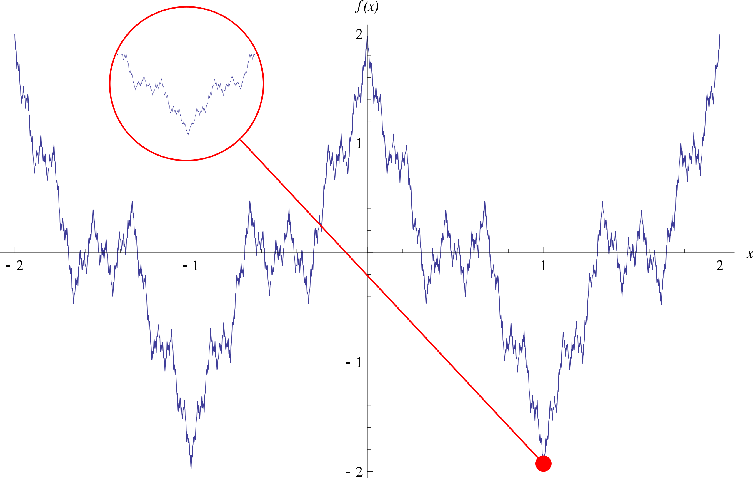
Image source: Wikipedia

What makes things worse is that in the realm of physics, you don’t even need to turn to such pathological examples for lack of rigour. In the department of physics, swapping the order of integrals is something you can always do, Taylor expansions always exist, and Dirac deltas are functions. At this point, “physical intuition” becomes akin to “hand-waving”.

A similar kind of failure mode is when the intuition fails not to mathematical rigour, but to the intrinsic (physical) unintuiveness of the physical system. Our physical intuitions are heavily influenced by our experiences and what we’re more familiar with - perhaps we need to turn to other kinds of intuition that are more abstract; an intuition that is gained simply by thinking about the equations a lot.

Despite these problems, I claim that physical intuition can still be useful. It really does just happen to be the case the many things in the physical world are sufficiently well-behaved that the aforementioned abuses of mathematics work, and have a ton of explanatory power¹³. Using physical intuition can help you make sense of phenomena in a deeper way, and guide lines of research.

Uniqueness

Another objection you might have is that physical intuition isn’t all that unique - other methods could give similar results, and analogous forms of reasoning exist in other fields. For instance, chess players tend to talk conceptually about “positional imbalances”, like “I need counterplay, so I’m going to go for a queenside minority attack”. Humans don’t decide on moves via alpha-beta tree search (or at least most don’t). If these are true, then what’s the case for using “physical intuition” rather than these other methods?

I think this is a pretty good point. It’s not immediately clear to me what the difference between different kinds of intuition is, probably because “physical intuition” is a rather nebulous concept. It seems to encapsulate geometric thinking, “imagining what’s going to happen”, determining the most important features of a system, and having a feel for what’s right or wrong - but these are just my impressions, and I think active physics researchers may tell you something different. If you have any thoughts on this, I’d love to hear about it!

Conclusions

In this post we’ve seen a couple of techniques by which one can leverage physical understanding in order to make progress on challenging problems:

• Understanding what the equation is describing and making simplifying assumptions, as in the ideal gas
• Checking dimensions, as in Rayleigh scattering
• Checking solutions and Taylor expansions, as in the uniformly charged disc
• Looking for symmetries, as in the heat equation

These have their pitfalls, but I think they can still be useful in many cases where 100% rigour isn’t necessary.

How might one go about developing these intuitions? I’m hesitant to give too much advice here, because I don’t consider myself to be much of an expert in this regard. However, prima facie it seems pretty reasonable that the main way to gain this intuition is to deliberately practise the techniques mentioned above - check your dimensions, think about the symmetries of the problem, and so on. If you’re feeling up to it, I’d encourage you to try and come up with examples of situations where the above techniques can be helpful too - I’ve listed a few relatively technical ones in the footnotes which you’re welcome to dig into deeper¹⁴. I imagine this is somewhat akin to how you might develop intuitions in maths, for instance by modifying theorem statements to try and understand why the conditions of the theorem are as stated.

I would love it if somebody with a deeper understanding of physics wrote a more advanced version of this post. It would also be nice if a mathematician wrote the dual version of this post, i.e. “what is mathematical intuition?”, targeted towards physicists. Perhaps a future version of me will write this, but no guarantees!

---